Examples

import cubedsphere and other helper packages

import numpy as np
import cubedsphere as cs

import matplotlib.pyplot as plt
import matplotlib.colors as mcolors
import cartopy.crs as ccrs  # optional, only needed for nicer projections

Specify folder of simulationdata

outdir_ascii = "/Volumes/EXTERN/Simulations/exorad/new_run/paper_runs/WASP-43b/run/"

Standard conservative regridding

Load data and regrid data

# open Dataset using xmitgcm (see docs for xmitgcm.open_mdsdataset for more details)
ds_ascii, grid = cs.open_ascii_dataset(outdir_ascii, iters=[41472000], prefix = ["T","U","V","W"])
# regrid dataset
regrid = cs.Regridder(ds_ascii, grid)
ds = regrid()
# (optional) converts wind, temperature and stuff
ds = cs.exorad_postprocessing(ds, outdir=outdir_ascii)

time needed to build regridder: 0.9600319862365723
Regridder will use conservative method

Minimal working example of a plot:

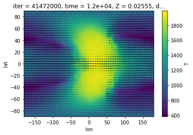
plt.figure()
# Select horizontal slice at latest time:
data = ds.isel(time=-1,Z=-20)
# Plot temperature:
data.T.plot()
# Overplot winds:
cs.overplot_wind(ds, data.U.values, data.V.values)
plt.show()

A littlebit nicer with cartopy:

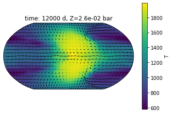
plt.figure()
ax = plt.axes(projection=ccrs.Robinson())
# Plot temperature:
data.T.plot(transform = ccrs.PlateCarree(), ax=ax)
# Overplot winds:
cs.overplot_wind(ds, data.U.values, data.V.values, ax=ax, transform=ccrs.PlateCarree(), stepsize=2)
ax.set_title('time: {:.0f} d, Z={:.1e} bar'.format(data.time.values,data.Z.values))
plt.show()

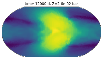
Utilizing the cubedsphere plot to do a comparison with the original (not regridded) data:

data_orig = ds_ascii.isel(time=-1,Z=-20)

fig, ax = plt.subplots(2,1, subplot_kw={"projection":ccrs.Robinson()})

# Do the plots
cs.plotCS(data_orig.T, data_orig, transform=ccrs.PlateCarree(), ax = ax[0])
ax[1].pcolormesh(data.lon, data.lat, data.T, transform = ccrs.PlateCarree())

ax[0].set_title('original data')
ax[1].set_title('regridded')

plt.show()

Zonal mean plots

For convenience, we will show an easy way on how to create a zonal mean wind plot

plt.figure()
zmean = ds.U.isel(time=-1).mean(dim='lon')
zmean.plot()
plt.yscale('log')
plt.ylim([700,1e-4])
plt.show()

From lon,lat to cubedsphere

We are now going to perform a second regridding (from already regridded original to cubedsphere)

# Add some info to the regridded dataset
reg_grid = regrid._build_output_grid(5, 4)
ds["lon_b"] = reg_grid["lon_b"]
ds["lat_b"] = reg_grid["lat_b"]

# Perform back regridding
regrid = cs.Regridder(ds, grid, input_type='ll')
ds_regback = regrid()

time needed to build regridder: 0.9572968482971191
Regridder will use conservative method

Congratulations! ds_regback is now again in cubedsphere coordinates!

plt.figure()
data_reg_back = ds_regback.isel(time=-1, Z=-20)
ax = plt.axes(projection=ccrs.Robinson())
ax.set_title('time: {:.0f} d, Z={:.1e} bar'.format(data.time.values,data.Z.values))
cs.plotCS(data_reg_back.T, data_reg_back, transform=ccrs.PlateCarree(), ax = ax)
plt.show()

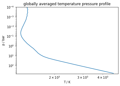
Calculate global averages

a globally averaged quatity \(\bar T\) can be calculated by

\(\bar T =\frac{\sum T\cdot\Delta A}{\sum{\Delta A}}\),

where \(\Delta A\) is the area of the grid cell.

plt.figure()
T_global = (ds.T.isel(time=-1)*ds.area_c).sum(dim=['lon','lat'])/ds.area_c.sum(dim=['lon','lat'])
plt.loglog(T_global, ds.Z)
plt.ylim(700,1e-4)
plt.title('globally averaged temperature pressure profile')
plt.ylabel('p / bar')
plt.xlabel('T / K')
plt.show()

Open userspecific files

Some packages (e.g., SPARC/MITgcm and exPERT/MITgcm) are not opensource and we therefore need to specify how we have to read the extra output generated by those codes.

This can be easily done using the extra_variables keyword, passed to open_mdsdataset from cs.open_ascii_dataset.

Extra variables can also be added to the codebase of the cubedsphere package. You can find already added exPERT/MITgcm variables here.

Note: Click here to see the options for all kwargs used to open datasets with xmitgcm.

We will now show an example of how we can load and plot the bolometric emission fluxes generated from the exPERT/MITgcm output.

# Note: Not needed, since already part of cubedsphere package, this is shown only to demonstrate how it works
extra_variables = dict(EXOBFPla=dict(dims=['k_p1', 'j', 'i'],
                                            attrs=dict(standard_name='EXOBFPla', long_name='Bolometric Planetary Flux',
                                                       units='W/m2')))

# open Dataset using xmitgcm (see docs for xmitgcm.open_mdsdataset for more details)
ds_ascii, grid = cs.open_ascii_dataset(outdir_ascii, iters=[41472000], prefix = ["EXOBFPla"], extra_variables=extra_variables)
# regrid dataset
regrid = cs.Regridder(ds_ascii, grid)
ds = regrid()
# (optional) converts wind, temperature and stuff
ds = cs.exorad_postprocessing(ds, outdir=outdir_ascii)

could not rename, got error: cannot rename 'T' because it is not a variable or dimension in this dataset
time needed to build regridder: 0.9598851203918457
Regridder will use conservative method

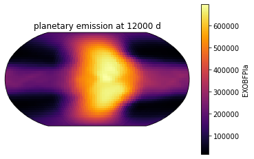
# Plot planetary emission:
plt.figure()
ax = plt.axes(projection=ccrs.Robinson())
ds.EXOBFPla.isel(time=-1, Zp1=-1).plot(transform = ccrs.PlateCarree(), ax=ax, cmap=plt.get_cmap('inferno'))
ax.set_title('planetary emission at {:.0f} d'.format(data.time.values))
plt.show()